Improving cloudless mosaic continuity across orbits

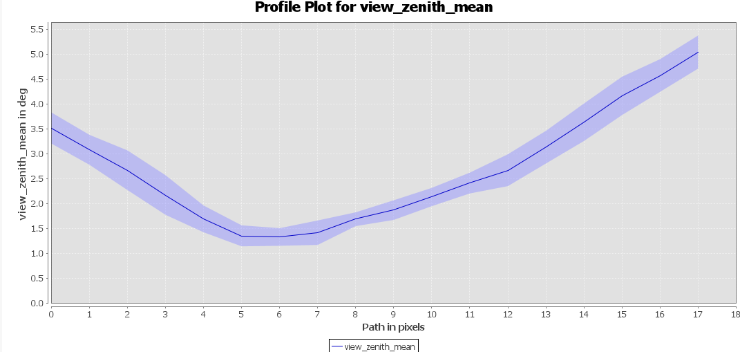
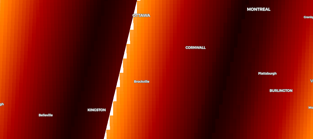
I am attempting to create large mosaics from Sentinel-2 for modeling vegetation structure. I have set up a custom script to create 20 meter resolution 5-band (2, 3, 4, 8, 11) cloudless mosaics filtered down to collections that occur during the summer months (June/July/August) of 2018, 2019, and 2020. This script is performing well in many places but there are cases where the orbit patterns are clearly visible in the output image. Here is a low-resolution preview that shows the problematic pattern:


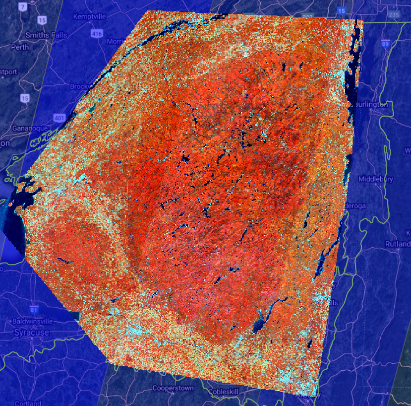
The nominal sentinel 2 orbit paths are displayed beneath the mosaic image, the darker blue areas are overlap zones between orbits. The stripe on the eastern edge of the mosaic is the most problematic, the source images appear to have very different spectral characteristics (lighter tones on eastern side, darker tones on western side).

Are there tweaks parameters in the Evalscript or in the request (i.e. date ranges, mosaicking settings, etc) that might help reduce the between-orbit stripe artifacts?

Input data request:

"data": [
        {
          "type": "S2L2A",
          "dataFilter": {
            "timeRange": {
              "from": "2018-06-15T00:00:00Z",
              "to": "2020-09-01T23:59:59Z"
            },
            "maxCloudCoverage": 50,
            "mosaickingOrder": "mostRecent"
          }
        }
      ]

Evalscript:

//VERSION=3

// copied from here:
// https://github.com/sentinel-hub/custom-scripts/blob/master/sentinel-2/cloudless_mosaic/L2A-first_quartile_4bands.js

function setup() {
  return {
    input: [{
      bands: [
        "B04", // red
        "B03", // green
        "B02", // blue
        "B08", // nir
        "B11", // swir
        "SCL" // pixel classification
      ],
      units: "DN"
    }],
    output: {
      bands: 5,
      sampleType: SampleType.UINT16
    },
    mosaicking: "ORBIT"
  };
}

// acceptable images are ones collected in summer months of 2018, 2019, 2020
function filterScenes(availableScenes, inputMetadata) {
  return availableScenes.filter(function(scene) {
    var m = scene.date.getMonth();
    var y = scene.date.getFullYear();
    var years = [2018, 2019, 2020];
    var months = [5, 6, 7]; // 0 indexed, 5 = June, 6 = July, 7 = August
    return months.includes(m) && years.includes(y);
  });
}

function getValue(values) {
  values.sort(function (a, b) {
    return a - b;
  });
  return getMedian(values);
}

// function for pulling first quartile of values
function getFirstQuartile(sortedValues) {
  var index = Math.floor(sortedValues.length / 4);
  return sortedValues[index];
}

// function for pulling median (second quartile) of values
function getMedian(sortedValues) {
  var index = Math.floor(sortedValues.length / 2);
  return sortedValues[index];
}


function validate(samples) {
  var scl = samples.SCL;

  if (scl === 3) { // SC_CLOUD_SHADOW
    return false;
  } else if (scl === 9) { // SC_CLOUD_HIGH_PROBA
    return false;
  } else if (scl === 8) { // SC_CLOUD_MEDIUM_PROBA
    return false;
  } else if (scl === 7) { // SC_CLOUD_LOW_PROBA
    // return false;
  } else if (scl === 10) { // SC_THIN_CIRRUS
    return false;
  } else if (scl === 11) { // SC_SNOW_ICE
    return false;
  } else if (scl === 1) { // SC_SATURATED_DEFECTIVE
    return false;
  } else if (scl === 2) { // SC_DARK_FEATURE_SHADOW
    // return false;
  }
  return true;
}

function evaluatePixel(samples, scenes) {
  var clo_b02 = [];
  var clo_b03 = [];
  var clo_b04 = [];
  var clo_b08 = [];
  var clo_b11 = [];
  var clo_b02_invalid = [];
  var clo_b03_invalid = [];
  var clo_b04_invalid = [];
  var clo_b08_invalid = [];
  var clo_b11_invalid = [];
  var a = 0;
  var a_invalid = 0;

  for (var i = 0; i < samples.length; i++) {
    var sample = samples[i];
    if (sample.B02 > 0 && sample.B03 > 0 && sample.B04 > 0 && sample.B08 > 0 && sample.B11 > 0) {
      var isValid = validate(sample);

      if (isValid) {
        clo_b02[a] = sample.B02;
        clo_b03[a] = sample.B03;
        clo_b04[a] = sample.B04;
        clo_b08[a] = sample.B08;
        clo_b11[a] = sample.B11;
        a = a + 1;
      } else {
        clo_b02_invalid[a_invalid] = sample.B02;
        clo_b03_invalid[a_invalid] = sample.B03;
        clo_b04_invalid[a_invalid] = sample.B04;
        clo_b08_invalid[a_invalid] = sample.B08;
        clo_b11_invalid[a_invalid] = sample.B11;
        a_invalid = a_invalid + 1;
      }
    }
  }

  var rValue;
  var gValue;
  var bValue;
  var nValue;
  var sValue;
  if (a > 0) {
    rValue = getValue(clo_b04);
    gValue = getValue(clo_b03);
    bValue = getValue(clo_b02);
    nValue = getValue(clo_b08);
    sValue = getValue(clo_b11);
  } else if (a_invalid > 0) {
    rValue = getValue(clo_b04_invalid);
    gValue = getValue(clo_b03_invalid);
    bValue = getValue(clo_b02_invalid);
    nValue = getValue(clo_b08_invalid);
    sValue = getValue(clo_b11_invalid);
  } else {
    rValue = 0;
    gValue = 0;
    bValue = 0;
    nValue = 0;
    sValue = 0;
  }
  return [rValue, gValue, bValue, nValue, sValue];
}

Hi @hrodman,

You are running into a physical problem which gets more and more complex as you dig deeper. I am speaking from experience here… :slight_smile:

Depending on where your pixel is located in the orbit, Sentinel-2 (or other polar-orbiting satellites) observes the surface with different viewing angles and the illumination geometries (this page illustrates the different angles) change also. I don’t know how much you know, so I apologise if this is obvious but I’ll put the information out there for others who are interested.

If all surfaces on Earth were lambertian, life for remote sensing specialists would be so much easier! Unfortunately, this is not the case and different surfaces scatter light very differently: with different intensities in different directions. The angular reflectance properties of a surface are quantified using the Bidirectional Reflectance Distribution Function (BRDF). See Crystal Schaaf’s very informative page on the subject, with nice visuals.

When you want to calculate radiative or physical properties of a surface on Earth using a satellite image that only gives you information about solar radiation reflected in one direction, you need to know how the surface reflects light in all directions, i.e. it’s BRDF (actually BRDF is not measurable, if you want to go down that rabbit hole, I recommend this excellent scientific paper). For example, to derive albedo (blue-sky albedo to be exact, albedo can mean different things) from optical satellite observations: if the surface was lambertian, you would just need to integrate the measured reflectance over the cosine of the viewing angle, but for non-lambertian surfaces, one would generally use a BRDF model of the observed surface. These models come under a variety of different forms: analytical, semi-empirical, 3D

But let’s get back to your problem…

Sentinel-2 provides reflectance measurements for a given viewing and illumination geometry.
From one side to the other of the orbit angular changes are quite small and gradual so you don’t notice their effect. Here is an example of the viewing zenith angle across a Sentinel-2 tile :

However, when you start stitching orbits, then you find yourself with a “jump” in angles, which causes you to notice the change visually. I pulled up an example of the satellite viewing angles for your AOI in EO Browser here, where you can see the “jump” from an orbit to another.

To answer your questions:

the source images appear to have very different spectral characteristics

Not quite, for the same surface type, the spectral characteristics will be very similar. However, since you are looking at the surface from 2 different angles, they appear different. See the following photo of the same forest taken from a helicopter (one picture with the sun behind the photographer, one picture facing the sun):

image
Photograph by Don Deering – BOREAS experimental region in Canada

Are there tweaks parameters in the Evalscript or in the request (i.e. date ranges, mosaicking settings, etc) that might help reduce the between-orbit stripe artifacts?

To avoid big steps between orbits to a maximum, I would recommend trying to keep the time period as narrow as you possibly can (if you stitch an image in June with one in December, you are obviously going to add the difference in surface characteristics to the existing problem). In the custom scripts repository, you can find a script that helps determine if there are enough cloud-free images in your time-range.

Apart from this, if you don’t normalise your reflectance, there is nothing much you can do. If you want to implement something yourself, you could always look at this paper: Examination of Sentinel-2A multi-spectral instrument (MSI) reflectance anisotropy and the suitability of a general method to normalize MSI reflectance to nadir BRDF adjusted reflectance - ScienceDirect

Please don’t hesitate to jump in for comments or observations on what I said.

Maxim

Thank you for the thorough response to my question, @maxim.lamare. I appreciate your explanation about the root causes of the apparent differences among images from different orbits and the relevant sources that you provided.

I have experimented with the allowable time window for the images and have observed the trade-off between width of acceptable time window and cloud-free performance. When I limit images to the month of June from years 2018, 2019, and 2020, there are clouds left behind in the mosaic presumably due to lack of available cloud-free images (this is a very cloudy place). When I expand the acceptable range of months to include June, July, and August, the cloud-free quality of the images is much greater but the orbit stripe patterns are more visible.

I would like to be able to apply some sort of normalization to mitigate the striping artifacts, are you aware of any example evalscripts that attempt this? Perhaps there are methods from the recently released global time series mosaic that could be helpful for this purpose?

While it would be ideal to have seamless-looking mosaics, it is possible that I can adapt my modeling process to account for these orbit patterns. How would you suggest adding a band to my output image that could describe the condition of each pixel in the source image? Maybe I could extract the viewZenithMean values as you displayed in the EO Browser example, maybe there is a different computation that would be appropriate? Any suggestions for how to pull this information into my evalscript would be appreciated.

Processing optical satellite imagery is always a question of trade-offs, indeed!

I would like to be able to apply some sort of normalization to mitigate the striping artifacts, are you aware of any example evalscripts that attempt this?

There are no Evalscripts that I know of that are available as of yet. The main problem is that you need apriori knowledge of the BRDF of the surface in order to normalise the data. If your surface was specific (i.e snow, or a distinct type of forest), it would be possible to implement a BRDF function in the Evalscript, that would take as inputs the reflectance and angular bands (they are provided with Sentinel-2).
Another option: the paper (very last link) in my previous post attempts to generate a generalised model with fixed parameters that could be applicable for a vast majority of surfaces (sacrificing some accuracy of course). I am currently working on implementing the approach as an Evalscript, but I’m doing as a hobby on the side so it will probably be a while before I get it out. Anybody that wants that Evalscript is most welcome to give me a hand! :grin:

Perhaps there are methods from the recently released global time series mosaic that could be helpful for this purpose?

The data wasn’t normalised in the global mosaic, and actually, you can notice striping in some areas. For example in South America here.

How would you suggest adding a band to my output image that could describe the condition of each pixel in the source image?

I can help you retrieve 3 relevant angular bands in your Evalscript: VZA (viewing zenith angle), SZA (solar zenith angle) and RAA (relative azimuth angle; the difference between solar azimuth angle and viewing azimuth angle). It’s not that straightforward because in the cloudless script you sort the pixels by reflectance value and retrieve the median / quartile. This means the script needs to be adapted to keep track of which acquisition the pixel comes from. I’ll try to get back to you early next week.

Maxim

@hrodman,

If it helps, here is an Evalscript that adds 3 bands to the Cloudless mosaic script that you posted in the first message of this thread. These bands correspond to the solar zenith angle, the viewing zenith angle and the relative azimuth angle (absolute difference between the solar azimuth and viewing azimuth angles).

To return the correct angle values for each pixel, I modified the script a little bit, but other methods can be implemented if you don’t like it. In the new version, rather than sorting each band from darkest to lightest and fetching the first or second quartile individually for each band, I sort the temporal stack based on Band 2 (Blue), return the index of the scene and use it to fetch the pixels for all other bands. This now means that for each pixel, all the bands correspond to the same scene.

//VERSION=3

// Cloudless mosaic, also returning the Viewing Zenith angles, Solar Zenith angles
// and Relative Azimuth angles (absolute difference bewtween Solar Azimuth & Viewing Azimuth angles).
// The pixels from all B02 (Blue) acquisitions are sorted from darkest to brightest,
// and the median or first quartile value and scene index are returned. This index is returned
// and used to fetch all other bands.

function setup() {
  return {
    input: [{
      bands: [
        "B04", // red
        "B03", // green
        "B02", // blue
        "B08", // nir
        "B11", // swir
        "SCL", // pixel classification
        "viewZenithMean", // VZA
        "sunZenithAngles", // SZA
        "viewAzimuthMean", // VAA
        "sunAzimuthAngles" // SAA
      ],
      units: "DN"
    }],
    output: {
      bands: 8,
      sampleType: SampleType.UINT16
    },
    mosaicking: "ORBIT"
  };
}

// acceptable images are ones collected in summer months of 2018, 2019, 2020
function filterScenes(availableScenes, inputMetadata) {
  return availableScenes.filter(function(scene) {
    var m = scene.date.getMonth();
    var y = scene.date.getFullYear();
    var years = [2018, 2019, 2020];
    var months = [5, 6, 7]; // 0 indexed, 5 = June, 6 = July, 7 = August
    return months.includes(m) && years.includes(y);
  });
}

function sortWithIndex(values){
  // Sort a list and return indices of original postions
  var vals_index = [];
  for (var i in values) {
    vals_index.push([values[i], i]);
  }
  vals_index.sort(function(left, right) {
    return left[0] < right[0] ? -1 : 1;
  });

  var indices = [];
  sorted = [];
  for (var j in vals_index) {
    sorted.push(vals_index[j][0]);
    indices.push(vals_index[j][1]);
  }
  
  return [sorted, indices];
}

function getValue(values) {
  
  // Sort and get indices
  sortedvals = sortWithIndex(values);
  
  return getMedian(sortedvals[0], sortedvals[1]);
}

// function for pulling first quartile of values
function getFirstQuartile(sortedValues) {
  var index = Math.floor(sortedValues.length / 4);
  return [sortedValues[index], originalIndices[index]];
}

// function for pulling median (second quartile) of values
function getMedian(sortedValues, originalIndices) {
  var index = Math.floor(sortedValues.length / 2);
  return [sortedValues[index], originalIndices[index]];
}


function validate(samples) {
  var scl = samples.SCL;

  if (scl === 3) { // SC_CLOUD_SHADOW
    return false;
  } else if (scl === 9) { // SC_CLOUD_HIGH_PROBA
    return false;
  } else if (scl === 8) { // SC_CLOUD_MEDIUM_PROBA
    return false;
  } else if (scl === 7) { // SC_CLOUD_LOW_PROBA
    // return false;
  } else if (scl === 10) { // SC_THIN_CIRRUS
    return false;
  } else if (scl === 11) { // SC_SNOW_ICE
    return false;
  } else if (scl === 1) { // SC_SATURATED_DEFECTIVE
    return false;
  } else if (scl === 2) { // SC_DARK_FEATURE_SHADOW
    // return false;
  }
  return true;
}

function evaluatePixel(samples, scenes) {
  var clo_b02 = [];
  var clo_b03 = [];
  var clo_b04 = [];
  var clo_b08 = [];
  var clo_b11 = [];
  var clo_sza = [];
  var clo_vza = [];
  var clo_raa = [];
  var clo_ind_invalid = [];
  var clo_b02_invalid = [];
  var clo_b03_invalid = [];
  var clo_b04_invalid = [];
  var clo_b08_invalid = [];
  var clo_b11_invalid = [];
  var clo_sza_invalid = [];
  var clo_vza_invalid = [];
  var clo_raa_invalid = [];
  var a = 0;
  var a_invalid = 0;

  for (var i = 0; i < samples.length; i++) {
    var sample = samples[i];
    if (sample.B02 > 0 && sample.B03 > 0 && sample.B04 > 0 && sample.B08 > 0 && sample.B11 > 0) {
      var isValid = validate(sample);

      if (isValid) {
        clo_b02[a] = sample.B02;
        clo_b03[a] = sample.B03;
        clo_b04[a] = sample.B04;
        clo_b08[a] = sample.B08;
        clo_b11[a] = sample.B11;
        clo_sza[a] = sample.sunZenithAngles;
        clo_vza[a] = sample.viewZenithMean;
        clo_raa[a] = Math.abs(sample.viewAzimuthMean - sample.sunAzimuthAngles);
        a = a + 1;
      } else {
        clo_b02_invalid[a_invalid] = sample.B02;
        clo_b03_invalid[a_invalid] = sample.B03;
        clo_b04_invalid[a_invalid] = sample.B04;
        clo_b08_invalid[a_invalid] = sample.B08;
        clo_b11_invalid[a_invalid] = sample.B11;
        clo_sza_invalid[a_invalid] = sample.sunZenithAngles;
        clo_vza_invalid[a_invalid] = sample.viewZenithMean;
        clo_raa_invalid[a_invalid] = Math.abs(sample.viewAzimuthMean - sample.sunAzimuthAngles);
        clo_ind_invalid[a_invalid] = i;
        a_invalid = a_invalid + 1;
      }
    }
  }

  var rValue;
  var gValue;
  var bValue;
  var nValue;
  var sValue;
  var bValInd;
  var szaValue;
  var vzaValue;
  var raaValue;
  

  if (a > 0) {
    
    // Rather than sort bands individually, we will use B02 for sorting
    // so that each pixel in all bands corresponds to the same scene
    bValInd = getValue(clo_b02);
    
    bValue = bValInd[0];
    rValue = clo_b04[bValInd[1]];
    gValue = clo_b03[bValInd[1]];
    bValue = clo_b02[bValInd[1]];
    nValue = clo_b08[bValInd[1]];
    sValue = clo_b11[bValInd[1]];
    szaValue = clo_sza[bValInd[1]];
    vzaValue = clo_vza[bValInd[1]];
    raaValue = clo_raa[bValInd[1]];

  } else if (a_invalid > 0) {
    bValInd = getValue(clo_b02_invalid);

    bValue = bValInd[0];
    rValue = clo_b04[bValInd[1]];
    gValue = clo_b03[bValInd[1]];
    bValue = clo_b02[bValInd[1]];
    nValue = clo_b08[bValInd[1]];
    sValue = clo_b11[bValInd[1]];
    szaValue = clo_sza[bValInd[1]];
    vzaValue = clo_vza[bValInd[1]];
    raaValue = clo_raa[bValInd[1]];

  } else {
    rValue = 0;
    gValue = 0;
    bValue = 0;
    nValue = 0;
    sValue = 0;
    szaValue = 0;
    vzaValue = 0;
    raaValue = 0;
  }
  
  // Returned band values need to be divided by 10000
  // Returned angle values need to be divided by 100
  var f = 100;
  return [rValue, gValue, bValue, nValue, sValue, szaValue * f, vzaValue * f, raaValue * f];
}

Maxim

@maxim.lamare thank you for the updated evalscript, I had been curious about methods for keeping track of the origin scene for each pixel so it is very helpful to see your approach. I will add the view/solar angles to my modeling process to see if some of the mosacking artifacts can be accounted for using that information.

I’m glad that helped. If you do get something interesting out of using the angles, I would be interested to hear about it :slight_smile:

Maxim

@maxim.lamare - have you made any progress on the Evalscript that uses the generalised model for BRDF correction? If you have a proof-of-concept I would be very interested in trying it out or contributing in some way!

@hrodman

I was on vacation the last two weeks, hence the delay in my response. I started working on this a bit but then put the idea on the back-burner as more important things came in.

Your post has motivated me to put together what I have done in a useful/reusable format. In my repository you should find all the elements to look into the problem yourself and maybe help me out a bit (at least do a sanity check in case I have made a mistake in the code). I will try moving forward in my spare-time in the future, but can’t guarantee when it will be done :slight_smile:

Don’t hesitate to let me know what you think of the approach!

Hi @hrodman ,

You can check out our latest blog post here: Looking at the right angle — an easy Sentinel 2 BRDF correction within Sentinel Hub | by Maxim Lamare | Sentinel Hub Blog | Apr, 2023 | Medium

Thank you for the discussions in this thread!

1 Like